Dynamic Load-balancing
Motivation
Load balance is one of the major challenges for the efficient supercomputer, especially for applications that exhibit workload variations. Load imbalance is an considerable impedance on the path towards higher degree of parallelism.
In particular, when load conditions changes dynamically, efficient mesh partitioning becomes an indispensible part of scalable design.
Goals
Fluid dynamic application in the field of industrial engineering require high degrees of parallelism to achieve an acceptable time to solution for a large problem size. Typical mesh-based approaches therefore rely on suitable partitioning strategies to distribute the computational load across the set of processes.
Therefore, an efficient load-balancing approach aims to achieve two goals:
- The work load should be distribute evenly
avoid waiting times of processing units
- At the same time the interfacing boundaries between partitions should be as small as possible.
minimize the time spend in communication
The optimization problem is NP-hard.
Two popular approaches
Graph-based Algorithm
A popular choice for graph-based partition is ParMetis.
ParMetis performing very well for mesh partition for a long time. However, since ParMetis require global knowledge of the mesh, with an increasing number of processes, graph-based partitioning algorithms seem to reach their scalability limits. The memory consumption grows linearly with the graph size, raising the need for alternatives which could avoid this problem. Such methods are based on space-filling curves (SFCs).
Space-filling curves (SFCs) based algorithm
SFCs reduce the partitioning problem from n dimension to one dimension. The remaining tast, the so-called 1D partitioning problem or chains-on-chains partitioning problem, is to decompose a 1D workload array into consecutive, balanced partitions.
Advantages
- Good Locality
SFCs map the 1D unit interval onto a higher dimensional space such that neighboring points on the unit interval are also neighboring points in the target space.
- Acceptable communication overhead
SFCs ignores the edges of full graph imformation. It relies on the spatial properties of the curve to ensure a reasonable partition shape. Tirthapura et al. demonstrated that the upper limit of expected remote accesses in SFC partiotned domains are acceptable [TSA06].
- Low memory using
Taking the good locality of SFCs, the global imformation (full graph information) needed by Graph-based algorithm can be abandoned. Thus, SFCs opens a path towards low-memory partitioning strategies.
Implementing SFC
The numerical approximation of wave equation is a hp-adaptive approach. That is, elements can split or merge (h-adaptive) according to therequired resolution. Also, they can raise or decrease the polynomial degree (p-adaptive) to adjust the convergence rate.
Due to the hp-adaptivity, different element can have differernt individual computation times, load imbalance is introuduce to this application. Re-meshing and domain partitioning are not avoidable.
With the help of a SFC, the 2D structured mesh partitioning problem can be reduced to a 1D chains-on-chains partitioning (CCP) problem. Knowing the index od an element, its neighbours indices can be computed locally.
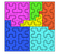
Hilbert Curve
There are many SFCs, for example Morton Curve (z-curve) and Hilbert Curve.
We choose Hilbert Curve as our SFC. Although Hilbert ordering is less efficient (with flip and rotation) than Morton Curve, Hilbert Curve brings out a better locality (no sudden “jump”).
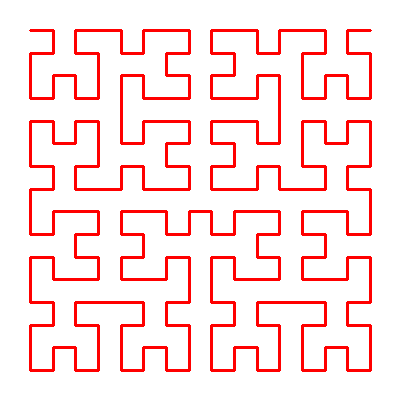
(Left Morton and right Hilbert)
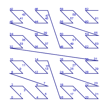
Static Grid Neighbour-finding algorithm
In Computation Fluid Dynamics, most of the cases, elements needs to exchange information (e.g. fluxes, velocity, pressure) with their neighbour. Thus, an effective way to locate your neighbours would cut down the computation time. When the neighbour is not stored locally, communication between processors is inevitable.

For instance, we are on element 31. The domain is partitioned into4 parts and each part is assigned to one processor. The integer coordingate of element 31 is (3, 4).
Therefore, its neighbours coordinates can be computed easily. Say we want to find its North and East neighbour, their coordinates are (3, 5) and (4, 4), respectively.
North neighbour: We can use our Hilbert-numbering function to map between coordinate and element index. Then (3, 5) corresponding to element 28. We successfully locate the Neighbour.
East neighbour: By using the same methond, we are able to compute the east neighbour index: 32. However, this element is not stored locally. Locate the processor who stores the target element is done by broadcasting the element range stored in each processor after the partitioning. And one-sided communication is invoked to warrent effective MPI message-changing.
Dynamic grid Neighbour-finding algorithm
When h-adaptivity is introduced to the code, element splits or merge according to the error indicator. Once an element split, it generates four identical “children” quadrants. The Octree partitioning is motivated by octree-based mesh generation.
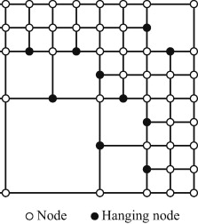
Neighbour-finding is achieved by using a global index (k, l, j, s) to identify element.
k: Root element number.
l: h-refinement level (split number).
j: child relative position inside a parent octant.
s: element state, can be used to determined Hilbert Curve orientation.
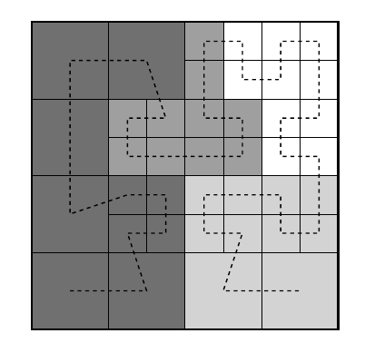
Partitioning stratigy
We consider a 2D mesh being represented by a one dimensional array using Hilbert Curve.
Implementation
We followed the CCP strategy described in [HKR+12]. The array has the length \(N\) which corresponding to the number of mesh cells. Weights are give as \(\omega_i\), where \(i\) corresponding to teh global index for each element. The weights represents the computation effort of each element. In fact, the load on each element due to fluid computation is \(O(N^4)\)[ZBMZ+18].
The task of the partition step is to decide which element to move to which processor. Here, we use \(p\) to denote the total number of processors, and every processor can be identified by a unique number called \(rank\). (\(0 \leqslant rank \leqslant p\))
We use an exclusive prefix sum to determine the partition.
For \(0 < I \leqslant N\) and \(prefix(0) = 0\). Local prefix sus are calculated, and the global offsets are adjusted afterwards using MPI_EXSCAN() collective with MPI_SUM as reduction operation. Then each prossessor has the global prefix sum for each of its local elements.
The ideal work load per partition is given by
Where \(\omega_{globalsum}\) is the global sum of all weights. Since the overall sum already computed through the prefix sum, we can use the last processor as a root to broadcast (MPI_BCAST) the \(\omega_{opt}\). Then the splitting positions between balanced partitions can be computed locally. There is no need further information changing to decide which element to move to which processor. The complete message changing for the partitioning only relies on two collective operation in MPI. Both collectives can be implemented efficiently using asymptotic running time ad memory complexity of \(O(logp)\).
Assuming homogeneous processors, ideal splitters are multiples of \(\omega_{opt}\), i.e., \(r \cdot \omega_{opt}\) for all integer \(r\) with \(1 \leqslant r < p\). The closest splitting positions between the actual elements to the ideal splitters can be found by comparing with the global prefix sum of each element.
The efficiency \(E\) of the distribution work is bounded by the slowest process, and thus cannot better than:
Exchange of Element
After the splitting positions are decided, elements needs to be relocated. The relocation, or exchange of elements is done via communication between processors. The challenge part is, though, the sender knows which element to send to which processor, the receiver does not know what they will receive.
Some application use a regular all-to-all collective operation to imform all processors about the their communication partners before doing teh actual exchange of the elements with an irregular all-to-all collective operation (e.g. MPI_Alltoallv).
Alternatively, elements can be propagated only between neighbour processors in an iterative fasion. This method can be benigh when the re-partitioning modifies an existing distribution of element only slightly. Unfortunately, worse cases can lead to \(O(p)\) forwarded messages.
In our implementation, One-sided Communication in MPI is invoked. In one-sided MPI operations, also known as RDMA or RMA (Remote Memory Access) operation. In RMA, the irregular communication patten can be handle easily without an extra step to determine how many sends-receives to issue. This makes dynamic communication easier to code in RMA, with the help of MPI_Put and MPI_Get.
References
- HKR+12
Daniel F. Harlacher, Harald Klimach, Sabine Roller, Christian Siebert, and Felix Wolf. Dynamic load balancing for unstructured meshes on space-filling curves. 2012 IEEE 26th International Parallel and Distributed Processing Symposium Workshops & PhD Forum, pages 1661–1669, 2012.
- TSA06
Srikanta Tirthapura, Sudip Seal, and Srinivas Aluru. A formal analysis of space filling curves for parallel domain decomposition. 2006 International Conference on Parallel Processing (ICPP‘06), pages 505–512, 2006.
- ZBMZ+18
Keke Zhai, Tania Banerjee-Mishra, David Zwick, Jason Hackl, and Sanjay Ranka. Dynamic load balancing for compressible multiphase turbulence. ArXiv, 2018.